Discretizing Continuous Attributes While Learning Bayesian Networksnpdf

1 Introduction

Bayesian networks (Pearl 1988; Koller and Friedman 2009) are often used to model uncertainty and causality, with applications ranging from decision-making systems (Kochenderfer et al. 2012) to medical diagnosis (Lustgarten et al. 2011)

. Bayesian networks provide an efficient factorization of the joint probability distribution over a set of random variables. It is common to assume that the random variables in a Bayesian network are discrete, since many Bayesian network learning and inference algorithms are unable to efficiently handle continuous variables. In addition, many of the commonly used Bayesian network software packages, such as Netica

(Norsys 1992–2009), SMILearn (Druzdzel 1999), and bnlearn (Scutari 2010), are geared towards discrete variables. However, many applications require the use of continuous variables, such as position and velocity in dynamic systems (Kochenderfer et al. 2010).

There are three common approaches to extending Bayesian networks to continuous variables. The first is to model the conditional probability density of each continuous variable using specific families of parametric distributions, and then to redesign Bayesian network learning and inference algorithms based on the parameterizations. One example of parametric continuous distributions in Bayesian networks is the Gaussian graphical model (Weiss and Freeman 2001).

The second approach is to use nonparametric distributions, such as particle representations and Gaussian processes (Ickstadt et al. 2010)

. Unlike parametric methods, nonparametric methods can often fit any underlying probability distribution given sufficient data. Parametric models have a fixed number of parameters, whereas the number of parameters in a nonparametric model grow with the amount of training data.

The third approach is discretization. Automated discretization methods have been studied in machine learning and statistics for many years

(Dougherty et al. 1995; Kerber 1992; Holte 1993; Fayyad and Irani 1993), primarily for classification problems. These methods search for the best discretization policy for a continuous attribute by considering its interaction with a class variable. It is common to discretize all continuous variables before learning a Bayesian network structure to avoid having to consider variable interactions, as the interactions and dependencies between variables in Bayesian networks introduce complexity. Prior work exists for discretizing continuous variables in naive Bayesian networks and tree-augmented networks (Friedman et al. 1997), but only a few discretization methods for general Bayesian networks have been proposed (Friedman and Goldszmidt 1996; Kozlov and Koller 1997; Monti and Cooper 1998; Steck and Jaakkola 2004).

A common discretization method for Bayesian networks is to split continuous variables into uniform-width intervals or by using field-specific expertise. A more principled method is the minimum description length (MDL) principle discretization (Friedman and Goldszmidt 1996). The MDL principle proposed by Rissanen (1978) states that the best model for a dataset is the one that minimizes the amount of information needed to describe it (Grünwald 2007). MDL methods trade off goodness-of-fit against model complexity to reduce generalization error. In the context of Bayesian networks, Friedman and Goldszmidt (1996) applied the MDL principle to determine the optimal number of discretization intervals for continuous variables and the optimal positions of their discretization edges. Their approach selects a discretization policy that minimizes the sum of the description length of the discretized Bayesian network and the information necessary for recovering the continuous values from the discretized data.

The optimal discretization policy of a single continuous variable under MDL can be found using dynamic programming in cubic runtime with the number of data instances. For Bayesian networks with multiple continuous variables, MDL discretization can be iteratively applied to each continuous variable. Only one variable is treated as continuous at a time, while all other continuous variables are treated as discretized based on an initial discretization policy or the discretization result from a previous iteration.

MDL discretization requires that the network structure be known in advance, but an iterative approach allows it to be incorporated into the structure learning process. Simultaneous structure learning and discretization alternates between traditional discrete structure learning and optimal discretization. Starting with some preliminary discretization policy, one first applies a structure learning algorithm to identify the locally optimal graph structure. One then refines the discretization policy based on the learned network. The cycle is repeated until convergence.

Results in this work suggest that the MDL method suffers from low sensitivity to discretization edge locations and returns too few discretization intervals for continuous variables. This is caused by MDL's use of mutual information to measure the quality of discretization edges. Mutual information, which is composed of empirical probabilities computed using event count ratios, varies less significantly with the positions of discretization edges than the method we suggest in this article.

MODL (Boullé 2006) is a Bayesian method for discretizing a continuous feature according to a class variable, which selects the model with maximum probability given the data. The MODL method uses dynamic programming to find the optimal discretization policy for a continuous variable given a discrete class variable, and has an runtime, where is the number of class variable instantiations. Lustgarten et al. (2011) suggest several formulations for the prior over models. The asymptotic equivalence between MDL and MODL on the single-variable, single-class problem was examined by Vitányi and Li (2000).

This paper describes a new Bayesian discretization method for continuous variables in Bayesian networks, extending prior work on single-variable discretization methods from Boullé (2006) and Lustgarten et al. (2011). The proposed method optimizes the discretization policy relative to the network and takes parents, children, and spouse variables into account. The optimal single-variable discretization method is derived in Section3, using a prior which reduces the discretization runtime to without sacrificing optimality. Section4 covers Bayesian networks with multiple continuous variables and Section5 covers discretization while simultaneously learning network structure. The paper concludes with a comparison against the existing minimum-description length (Friedman and Goldszmidt 1996) method on real-world datasets in Section6.

2 Preliminaries

This section covers the notation used throughout the paper to describe discretization policies. This section also provides a brief overview of Bayesian networks.

2.1 Discretization Policies

Let be a continuous variable and let be a specific instance of . A discretization policy for is a mapping from to such that

The discretization policy discretizes into intervals. Let the samples of in a given dataset be sorted in ascending order, , and let the unique values be . The index of the last occurrence of in is denoted .

The discretization edges mark the boundaries between discretization intervals. In this paper, as with MODL, they are restricted to the midpoints between unique ascending instances of . Thus, each edge equals for some . Two useful integer representations of can be written

where , , , and . The representation is the number of instances before every discretization edge whereas the representation is the number of instances within each discretization interval.

2.2 Bayesian Networks

A Bayesian network over random variables is defined by a directed acyclic graph

whose nodes are the random variables and a conditional probability distribution for each node given its parents. The edges in a Bayesian network represent probabilistic dependencies among nodes and encode the Markov property: each node

is independent of its non-descendants given its parents in . The children of node are denoted .

When discussing the discretization of a particular continuous variable , let be the th parent of , let be the th child of , and let be the set of spouses of associated with the th child.

3 Single Variable Discretization

This section covers the discretization of a single continuous variable in a Bayesian network where all other variables are discrete. An optimal discretization policy for a dataset maximizes for some prior and likelihood .

3.1 Priors and Objective Function

Let be the subset of the training data corresponding to variable subset . Four principles for the optimal discretization policy enable the formulation of and , where is the subset of the dataset for all variables but , and the probability of the data associated with the target variable, , is already captured in . The four principles, which can be considered an extension of the priors in MODL and Lustgarten et al. (2011) to Bayesian networks, are:

1. The prior probability of a discretization edge between two consecutive unique values

   and is proportional to their difference:

   where is the largest number of intervals among discrete variables in 's Markov blanket. This encourages edges between well-separated values over edges between closely packed samples.

2. For a given discretization interval, every distribution over the parents of is equiprobable.

3. For each pair and a given discretization interval, every distribution over given an instance of is equiprobable.

4. The distributions over given each child, parent, and spouse instantiation are independent.

From the first principle one obtains the prior over the discretization policy:

The Bayesian network graph structure causes the likelihood term to factor according to 's Markov blanket:

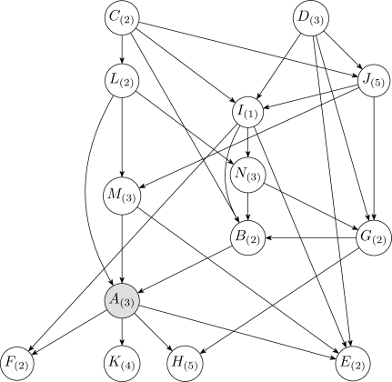
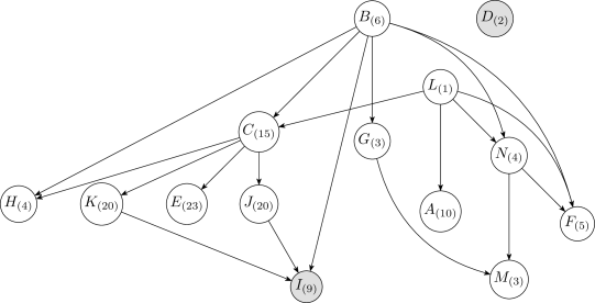
For example, in Figure1, factors according to

Figure 1: Factorization of .

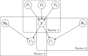
The concept behind the factorization is also the motivation behind forward sampling in a Bayesian network. The parents of are independent of the children given . The parents are not necessarily individually independent, and thus the parental term cannot be factored further. The children of are similarly independent given and the corresponding spouses, leading to their factored product . Each component in the decomposition can be evaluated given a discretization policy and a dataset.

3.1.1 Evaluation of

Let be the number of instantiations of the parents of , and let be the number of instances of within the th discretization interval of given the th parental instantiation. Note that . It follows that

The two factors on the right hand side come from the second principle: all distributions of values of the parents of in a given interval are equiprobable. The fourth principle is that the distributions for each interval are independent, so the factors can be multiplied together.

3.1.2 Evaluation of

Let be the number of instantiations of the th child of , let be the number of instantiations of the th spouse set , and let be the number of instances of in the th discretization interval of given the th instantiation of and the th instantiation of . Let . Note that for all . It follows that

The two factors on the right hand side come from the third principle: all distribution of values of in a given interval and with a given value of are equiprobable. According to the fourth prior, these distributions are independent from each other, and one can thus take their product. If , then Equation8 is equivalent to

where is the number of instances of in the th discretization interval of given the th instantiation of .

The objective function can be formulated given equations 4 ,5,7,8 and9. The log-inverse of is minimized for computational convenience:

3.2 Single-Variable Discretization Algorithm

The procedure used to minimize the objective function involves dynamical programming. Note that because the objective function is cumulative over intervals, if a partition of is an optimal discretization policy, then any subinterval is optimal for the corresponding subproblem. It follows that dynamic programming can be used to solve the optimization problem exactly.

Precomputation reduces runtime. Hence, is computed first for each interval starting from to for all , satisfying :

The calculation of for all has a runtime, where and are the number of child and parent variables respectively, is the largest cardinality of variables in 's Markov blanket, and .

The optimization problem over Equation10 can now be solved. The dynamic programming procedure is shown in Algorithm1. It takes three inputs: , the continuous variable; , the joint data instances over all variables sorted in ascending order according to ; and , the network structure. The runtime of Algorithm1 is also because the runtime of the dynamic programming procedure is less than the runtime for computing . As will be discussed in Section6, the MDL discretization method has a runtime of , which includes an extra term. The Bayesian discretization method is quadratic in the sample count , whereas the MDL discretization method is cubic.

Algorithm1 is guaranteed to be optimal. For faster methods with suboptimal results, see Boullé (2006).

functionDiscretizeOne( , , )

an matrix such that ; can be precomputed

the largest cardinality over all discrete variables in the Markov blanket of

the optimal objective value computed over samples to

5: the discretization policy for the subproblem over samples to

for and

for to do

if then

10:

else

for to do

15: if then

else

if then

20:

return

Algorithm 1 Discretization of one continuous variable in a Bayesian network

4 Multi-Variable Discretization

The single-variable discretization method can be extended to Bayesian networks with multiple continuous variables by iteratively discretizing individual variables. The discretization process for a single variable requires that all other variables be discrete. The iterative approach uses an initial discretization policy in order to start the process which assigns equal-width intervals to each continuous variable, where is the largest number of intervals of initially discrete variables in the network.

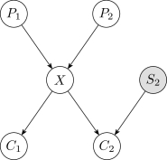
After the initial discretization, the one-variable discretization method is iteratively applied over each continuous variable in reverse topoligical order, from the leaves to the root. Reverse topological order has the advantage of relying on fewer initial discretizations of the continuous variables during the first pass. For example, in the network of Figure2, if is the only discrete variable, then the discretization of involves both and , whereas the discretization of only involves .

Figure 2: An example network.

The algorithm is terminated when the number of discretization intervals and their associated edges converge for all variables, and a maximum number of complete passes is enforced to prevent infinite iterations when convergence does not occur. The algorithm typically converges within a few passes when tested on real-world data.

The pseudocode for the multi-variable discretization procedure is shown in Algorithm2. It requires four inputs:

, a dataset of samples from the joint distribution;

, the fixed network structure; , the set of all continuous variables in reverse topological order, and , an upper bound on the number of complete passes.

functionDiscretizeAll( , , , )

the discretization policies for each in

the dataset discretized according to

5: for such that and is the discretized version of do

equal-width discretization of with intervals

while has not converged and do

10:          increment

for such that do

15: return

Algorithm 2 Discretization of multiple continuous variables

5 Combining Discretization with Structure Learning

It is often necessary to infer the structure of a Bayesian network from data. Three common approaches to Bayesian network structure learning are constraint-based, score-based, and Bayesian model averaging (see Koller and Friedman 2009, chap. 18). This work uses the K2 structure learning algorithm (Cooper and Herskovits 1992), a frequently used score-based structure learning method. Score-based structure learning methods over discrete variables commonly evaluate candidate structures according to their likelihood against a dataset . In practice, one maximizes the log-likelihood, also known as the Bayesian score, (Cooper and Herskovits 1992).

For a Bayesian network over discrete and discretized variables , represents the number of instantiations of , and represents the number of instantiations of the parents of . If has no parents, then . The Bayesian score is:

where is the gamma function, is a Dirichlet parameter and is the observed sample count for the th instantiation of and the th instantiation of . In the equation above,

The space of acyclic graphs is superexponential in the number of nodes; it is common to rely on heuristic search strategies

(Koller and Friedman 2009). The K2 algorithm assumes a given topological ordering of variables and greedily adds parents to nodes to maximally increase the Bayesian score. A fixed ordering ensures acyclicity but does not guarantee a globally optimal network structure. K2 is typically run multiple times with different topological orderings, and the network with the highest likelihood is retained.

Traditional Bayesian structure learning algorithms require discretized data, whereas the proposed discretization algorithm requires a known network structure. The discretization methods can be combined with the K2 structure learning algorithm (Cooper and Herskovits 1992) to simultaneously perform Bayesian structure learning and discretization of continuous variables.

The proposed algorithm alternates between K2 structure learning and discretization. The dataset is initially discretized as was described in Section4, and K2 is run to obtain an initial network structure. The affected continuous variables are rediscretized every time an edge is added by K2. The resulting discretization policies are used to update the discretized dataset, and the next step of the K2 algorithm is executed. This cycle is repeated until the K2 algorithm converges.

This procedure is given in Algorithm3, and takes five inputs: , a dataset of samples from the joint distribution; , the set of all continuous variables; order, a permutation of the variables in ; , an upper bound on the number of parents per node; and , an upper bound on the number of complete passes. The upper bound on the number of parents is common practice, and is used to prevent computing conditional distributions with excessively large parameter sets. The function in Algorithm3 computes a component of the Bayesian score (Equation 12 ):

functionLearn_DVBN( , , order, , )

the number of variables in the Bayesian network

the discretization policies for each in

5: the dataset discretized according to

the initially edgeless graph structure

for such that and is the discretized version of do

equal-width discretization of with intervals

10: for to do

(Equation14)

         OKToProceed true

while OKToProceed and do

an element from the set

15:

if then

sorted in reverse-topological order given

20: DiscretizeAll( , , , )  (see Algorithm2)

else

                  OKToProceed false

return ,

Algorithm 3 Learning a discrete-valued Bayesian network

It is common practice to run K2 multiple times with different variable permutations and to then choose the structure with the highest score. As such, Algorithm3 is run multiple times with different variable permutations and the discretized Bayesian network with the highest score is retained.

6 Experiments

This section describes experiments conducted to evaluate the Bayesian discretization method. All experiments were run on datasets from the publically available University of California, Irvine machine learning repository (Lichman 2013). Variables are labeled alphabetically in the order given on the dataset information webpage. In the figures that follow, shaded nodes correspond to initially discrete variables and the subscripts indicate the number of discrete instantiations.

Two experiments were conducted on each dataset. The first experiment compares the performance of the Bayesian and MDL discretization methods on a known Bayesian network structure. The structure was obtained by discretizing each continuous variable into uniform-width intervals, where is the median number of instantiations of the discrete variables, and using the structure with the highest Bayesian score from runs of the K2 algorithm with random topological orderings. The second experiment compares the same methods applied when simultaneously discretizing and learning network structure.

The discretizations are compared using the mean cross validated log-likelihood of the data given the Bayesian network and discretization policies . Note that all log-likelihoods shown have been normalized by the number of data samples. The log-likelihood has two components,

where is the original test dataset and is the test dataset discretized according to .

The log-likelihood of the discretized dataset given the Bayesian network is

where and are the Dirichlet prior counts and observed counts in the training set for , and is the set of observed counts in the test set . All experiments used a uniform Dirichlet prior of for all , , and .

The log-likelihood of the original dataset given the discrete dataset is

Note that and

. The mean cross-validated log-likelihood is the mean log-likelihood on the witheld dataset among cross-validation folds, and acts as an estimate of generalization error. Ten folds were used in each experiment.

The method for computing the MDL discretization policy is similar to the method for the Bayesian method. For a Bayesian network with a single continuous variable , the MDL objective function is

where is the mutual information between two discrete variable sets and , , and is the discretized version of .

The global minimum of Equation18 can be found using dynamic programming. For a given Bayesian network, the first three terms only depend on the number of discretization intervals and the fourth term is cumulative over the intervals. Hence, if is a MDL optimal discretization policy with intervals, then is a MDL optimal discretization policy for the corresponding subproblem with intervals. This procedure takes runtime . All variables are defined in Section 3.2. Therefore, the runtime of the proposed method in this paper is shorter than the MDL discretization method by , since the former has a more efficient form of dynamical programming. For faster methods of MDL discretization with suboptimal results, see Friedman and Goldszmidt (1996).

Note that the preliminary discretization and the discretization order of variables can be arbitrary for the MDL discretization method, as stated in the original work (Friedman and Goldszmidt 1996). In order to make a fair comparison between the Bayesian and MDL method, the preliminary discretization and the discretization order follows the same procedure as in Section 4.

6.1 Dataset 1: Auto MPG

The Auto MPG dataset contains variables related to the fuel consumption of automobiles in urban driving. The dataset has samples over eight variables, not including six instances with missing data. Three variables are discrete: , , and , with , , and instantiations respectively.

6.1.1 Discretization with Fixed Structure

The Bayesian and MDL discretization methods were tested on the Auto MPG data using the network shown in Figure3. This structure was obtained by initially discretizing each continuous variable into five uniform-width intervals, where five is the median cardinality of the discrete variables, and then taking the structure with highest likelihood from runs of K2.

Figure 3: Bayesian network structure obtained from running K2 on the initially uniformly discretized Auto MPG dataset.

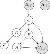
Table1 lists the discretization edges and mean log-likelihoods under -fold cross validation of the discrete Bayesian network resulting from the two discretization methods. The MDL method does not produce any discretization edges, assigning one continuous interval to each continuous variable, and produces the result with the lower likelihood. The reason why MDL produces fewer discretization edges is discussed in Section6.4. Two examples that MDL produces comparble results to the Bayesian method are given in the Appendix.

Table 1: Discretization result of the Auto MPG dataset with fixed structure from Figure3. The first five rows list the discretization edges and the last row lists the mean cross-validated log-likelihood; positive values are better.

Figure4 shows the marginal probability density for variables and under the Bayesian discretization policy overlaid with the original Auto MPG data. The resulting probability density is a good match to the original data.

Figure 4: Comparison of the Bayesian discretization policy for variables and to the original Auto MPG data learned with a fixed network. The marginal probability density closely matches the data.

6.1.2 Discretization while Learning Structure

In this experiment, the network structure was not fixed in advance and was learned simultaneously with the discretization policies. Figure5 shows a learned Bayesian network structure and the corresponding numbers of intervals after discretization for each continuous variable. This result was obtained by running Algorithm3 fifty times using the Bayesian method and choosing the structure with the highest K2 score (Equation 12 ).

Figure 5: The discrete-valued Bayesian network learned from the Auto MPG dataset using the Bayesian method.

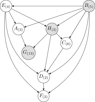
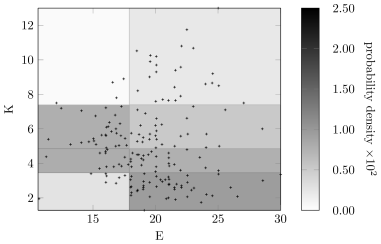
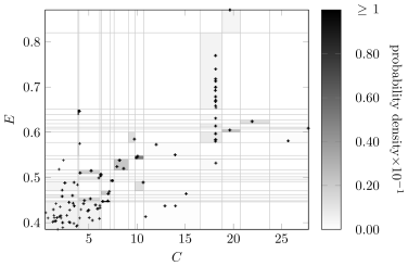
Figure6 compares the Bayesian discretizaton policy for variables and in the learned network with the original Auto MPG data. The color of a discretized region indicates the marginal probability density of a sample from being drawn from that region. Although there are fewer discretization edges for and in the learned network, the marginal distribution is still captured. The discretization policy will vary as the network structure changes, and it still produces high-quality discretizations.

Figure 6: Comparison of the Bayesian discretization policy for variables and to the original Auto MPG data learned simultaneously with the network structure. Although the number of discretization edges is less than those in Figure4, the probability distribution still closely matches the original data.

6.2 Dataset 2: Wine

The Wine dataset contains variables related to the chemical analysis of wines from three different Italian cultivars. The dataset has samples over fourteen variables. Variable is the only discrete variable and has three instantiations.

6.2.1 Discretization with Fixed Structure

The Bayesian and MDL discretization methods were tested on the Wine data using the network shown in Figure7. This structure was obtained by initially discretizing each continuous variable into three uniform-width intervals, where three is the median cardinality of the discrete variables, and then taking the structure with highest likelihood from runs of K2.

Table2 lists the discretization edges and mean log-likelihoods under -fold cross validation of the Bayesian network resulting from each discretization method. The Bayesian method outperforms the MDL method in likelihood by a significant margin. The MDL method creates significantly fewer discretization edges.

Some discretization edges appear in all three discretization methods, such as and for variable and for variable . This indicates sufficiently MDL indeed can find some important discretization edges, but it is not sensitive to find more edges.

Figure 7: Bayesian network structure obtained from running K2 on the initially uniformly discretized Wine dataset.

Table 2: Results from discretization of the Wine MPG dataset with fixed structure. Bold discretization edges were identified by both methods.

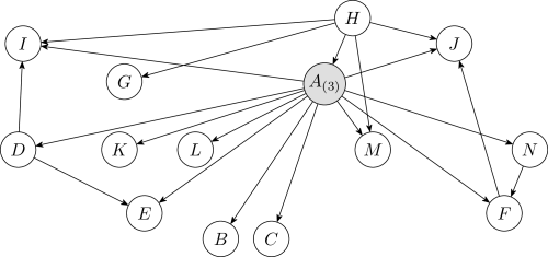
Figure8 compares the Bayesian and MDL discretizaton policies for variables and with the original Wine data. The discretization edges for and for appear in both plots. The MDL method does not use enough intervals for discretization. Relative sensitivities of each method to the input data is discussed in Section6.4.

Figure 8: Comparison of the discretization policies for variables and obtained using the Bayesian and MDL methods.

6.2.2 Discretization while Learning Structure

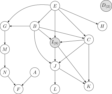
Figure9 is the discrete-valued Bayesian network learned from the Wine dataset, obtained by running Algorithm3 fifty times. A comparison of Figures9 and 7 show that the Bayesian network learned during the discretization process has more edges than the network learned on the initially discretized data. When a network is learned along with discretization, the algorithm has more freedom to adjust the structure and the discretization policy simultaneously to identify useful correlations and produce a denser structure.

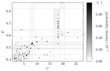
Figure10 shows the discretization policy for variables and obtained with the Bayesian method. The discretization edge also appears in both discretization policies from the fixed network (Figure8). This suggests that discretization edges can be robust against network structure. Furthermore, the discretization edge at in the fixed-structure case is missing in the learned structure. This is caused by having twice as many parents in the learned network structure. The more parents a variable has, the fewer discretization intervals it can to support, as the number of sufficient statistics required to define the resulting distribution increases exponentially with the number of parents.

Figure 9: The discrete-valued Bayesian network learned from the Wine dataset using the Bayesian method.

Figure 10: The discretization policy for variables and on the learned network. The discretization edge also appears in the policies for the fixed network.

6.3 Dataset 3: Housing

The Housing dataset contains variables related to the values of houses in Boston suburbs. The dataset has samples over fourteen variables. Only variables and are discrete-valued, with and instantiations, respectively. Despite their being continuous, several variables in the Housing dataset possess many repeated values. The following experiments were conducted with a maximum of three parents per variable to prevent running out of memory when running MDL.

6.3.1 Discretization with Fixed Structure

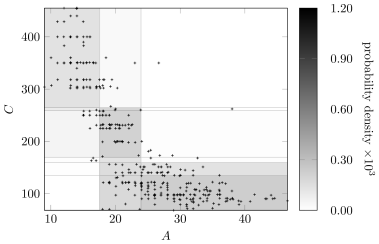
The Bayesian network structure in Figure11 was obtained by initially discretizing each continuous variable into five uniform-width intervals and then running the K2 algorithm times and choosing the network with the highest likelihood. Table3 shows the numbers of interval after discretization for each continuous variable and the log-likelihood of the dataset based on each discretization method. MDL method does not produce any discretization edges for most variables. The relative weighting of each method's objective function will be discussed in Section6.4.

Figure 11: Bayesian network structure obtained from running K2 on the initially uniformly discretized Housing dataset.

Table 3: Discretization policy summary of the Housing dataset based on the fixed network structure shown. The first twelve rows show the numbers of discretization intervals and the last row is the mean cross-validated log-likelihood.

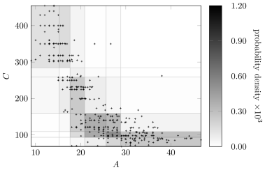
Figures12 and 13 show the discretization policy learned using the Bayesian approach on the fixed network shown in Figure11. The scatter points in Figure12 were jittered to show the quantity of repeated values for variables and . Each repeated point forms a single discrete region, thereby encouraging discretization. In contrast, the samples for are well spread out, resulting in fewer discretization regions and larger discretization intervals.

Figure 12: The discretization policies for variables and learned using the Bayesian approach on the fixed network. The scatter points were jittered to reveal the repeated values in the dataset. Values perfectly repeated in and lead to high correlation and concentrated densities in the marginal distribution.

6.3.2 Discretization while Learning Structure

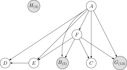
Figure14 shows a learned Bayesian network structure and the corresponding numbers of intervals after discretization for each continuous variable. Variable is neighborless in both the learned and fixed networks. The continuous variables , , and , which are all connected through , have many discretization intervals. Typically, when discretizing a variable, the expected number of discretization intervals is close to the highest cardinality among variables in its Markov blanket. This naturally leads to clusters of variables with many discretization intervals.

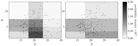
Figures15 and 16 show the discretization result for variables in the network shown in Figure14. Again, variable and have many discretization edges due to repeated values. Although the number of intervals after discretization on is less the number in Figure13, it still captures the distribution of the raw data along with the discretization edges for .

Figure 13: The discretization policies for variables and learned using the optimal Bayesian approach on the fixed network shown in Figure11. The values for variable are not as repeated, thus producing fewer discretization intervals than .

Figure 14: The discrete-valued Bayesian network learned from the Housing dataset using the optimal Bayesian method.

Figure 15: The discretization policy for variables and on the learned network in Figure14. The large number of discretization edges are due to repeated values in and . The two regions at and are color-saturated due to the high concentration of repeated values.

Figure 16: The discretization policy for variables and on the learned network in Figure14. There are fewer discretization intervals for than for the fixed network structure in Figure13, but the discretization result still closely models the raw data.

6.4 Discussion

Figure 17: A simple Bayesian network used to demonstrate the sensitivity of each method.

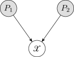
To qualitatively assess the sensitivity of each method to the number and position of discretization intervals, consider the Bayesian network in Figure17, where is continuous and and are discrete. If and , then the corresponding objective functions for the discretization methods are:

where and are constant over discretizations, is the number of discretization intervals, and is the mutual information based on estimated probabilities. Note that the third term of had been approximated using (see Equation18) in the original work by Friedman and Goldszmidt (1996), but it is written here without that approximation.

The penalty terms tend to increase with the number of discretization intervals; the edge position terms vary with the position and number of the discretization edges. A policy with a larger number of discretization edges is only optimal if the edge position term varies enough with respect to the penalty term in order to produce a local minimum of sufficiently low value.

The value of the edge position term for MDL is primarily determined by the mutual information, which varies less severely than the corresponding terms in the Bayesian method. The MDL term uses empirical probability distributions based off of ratios of counts, whereas the Bayesian method uses factorial terms, and thus the MDL method varies less. The MDL method is therefore less sensitive to the discretization edges. This sensitivity gives rise to the relative performance of the two methods in the experiments conducted above.

7 Conclusion

This paper introduced a principled discretization method for continuous variables in Bayesian networks with quadratic complexity instead of the cubic complexity of other standard techniques. Empirical demonstrations show that the proposed method is superior to the state of the art. In addition, this paper shows how to incorporate existing methods into the structure learning process to discretize all continuous variables and simultaneously learn Bayesian network structures. The proposed method was incorporated and its superior performance was empirically demonstrated. Future work will investigate edge positions at locations other than the midpoints between samples and will extend the approach to cluster categorical variables with very many levels. All software is publicly available at

github.com/sisl/LearnDiscreteBayesNets.jl.

References

• Boullé (2006) Marc Boullé. MODL: A Bayes optimal discretization method for continuous attributes. Machine Learning, 65:131–165, 2006.
• Cooper and Herskovits (1992) Gregory F. Cooper and Edward Herskovits. A Bayesian method for the induction of probabilistic networks from data. Machine Learning, 9(4):309–347, October 1992.
• Dougherty et al. (1995) J. Dougherty, R. Kohavi, and M. Sahami. Supervised and unsupervised discretization of continuous features. In International Conference on Machine Learning (ICML). Morgan Kaufman, 1995.
• Druzdzel (1999) Marek J. Druzdzel. SMILE: Structural modeling, inference, and learning engine and GeNIe: a development environment for graphical decision-theoretic models. In

  National Conference on Artificial Intelligence (AAAI)

  , pages 902–903, July 1999.
• Fayyad and Irani (1993) U.M. Fayyad and K.B. Irani. Multi-interval discretization of continuous-valued attributes for classification learning. In International Joint Conference on Artificial Intelligence (IJCAI), pages 1022–1027, 1993.
• Friedman and Goldszmidt (1996) N. Friedman and M. Goldszmidt. Discretizing continuous attributes while learning Bayesian networks. In International Conference on Machine Learning (ICML). Morgan Kaufman, 1996.
• Friedman et al. (1997) N. Friedman, D. Geiger, and M. Goldszmidt.

  Bayesian network classifiers.

  Machine Learning, 29:131–163, 1997.
• Grünwald (2007) P. D. Grünwald. Minimum Description Length Principle. MIT Press, 2007.
• Holte (1993) R.C. Holte. Very simple classification rules perform well on most commonly used datasets. Machine Learning, 11:63–90, 1993.
• Ickstadt et al. (2010) K. Ickstadt, B. Bornkamp, M. Grzegorczyk, J. Wieczorek, M. R. Sheriff, H. E. Grecco, and E. Zamir. Nonparametric Bayesian network. Bayesian Statistics, 9:283–316, 2010.
• Kerber (1992) R. Kerber. ChiMerge: Discretization of numeric attributes. In National Conference on Artificial Intelligence (AAAI), pages 123–128. AAAI Press, 1992.
• Kochenderfer et al. (2010) Mykel J. Kochenderfer, Matthew W. M. Edwards, Leo P. Espindle, James K. Kuchar, and Daniel J. Griffith. Airspace encounter models for estimating collision risk. AIAA Journal of Guidance, Control, and Dynamics, 33(2):487–499, 2010.
• Kochenderfer et al. (2012) Mykel J. Kochenderfer, Jessica E. Holland, and James P. Chryssanthacopoulos. Next-generation airborne collision avoidance system. Lincoln Laboratory Journal, 19(1):17–33, 2012.
• Koller and Friedman (2009) D. Koller and N. Friedman. Probabilistic Graphical Models: Principles and Techniques. MIT Press, 2009.
• Kozlov and Koller (1997) A.V. Kozlov and D. Koller. Nonuniform dynamic discretization in hybrid networks. In Conference on Uncertainty in Artificial Intelligence (UAI), pages 314–325, 1997.
• Lichman (2013) M. Lichman. UCI machine learning repository, 2013. URL http://archive.ics.uci.edu/ml.
• Lustgarten et al. (2011) J. L. Lustgarten, S. Visweswaran, V. Gopalakrishnan, and G. F. Cooper. Application of an efficient Bayesian discretization method to biomedical data. BMC Bioinformatics, 12(1):309, 2011.
• Monti and Cooper (1998) S. Monti and G.F. Cooper. A multivariate discretization method for learning Bayesian networks from mixed data. In Conference on Uncertainty in Artificial Intelligence (UAI), pages 404–413, 1998.
• Norsys (1992–2009) Norsys. Netica Bayesian network software package, 1992–2009. URL http://www.norsys.com.
• Pearl (1988) J. Pearl. Probabilistic Reasoning in Intelligent Systems: Networks of Plausible Inference. Morgan Kaufman, 1988.
• Rissanen (1978) J. Rissanen. Modeling by shortest data description. Automatica, 14(5):465–471, 1978.
• Scutari (2010) Marco Scutari. Learning Bayesian networks with the bnlearn R package. Journal of Statistical Software, 35(3):1–22, 2010. URL http://www.jstatsoft.org/v35/i03/.
• Steck and Jaakkola (2004) Harald Steck and Tommi S Jaakkola. Predictive discretization during model selection. In Pattern Recognition, volume 3175 of Lecture Notes in Computer Science, pages 1–8. Springer, 2004.
• Vitányi and Li (2000) Paul Vitányi and Ming Li. Minimum description length induction, Bayesianism, and Kolmogorov complexity. Information Theory, IEEE Transactions on, 46(2):446–464, 2000.
• Weiss and Freeman (2001) Y. Weiss and W. T. Freeman. Correctness of belief propagation in gaussian graphical models of arbitrary topology. Neural Computation, 13(10):2173–2200, 2001.

Appendix

This section gives two examples of Bayesian networks where MDL produces comparable results to the Bayesian method. The first example used the Auto MPG dataset. Instead of testing on the network obtained using initially uniform discretization and structure learning, the tested network is obtained by Algorithm 3, which can be considered better-structured than the network in Figure 3. The second example is on the Iris dataset (Lichman 2013). In the work of Friedman and Goldszmidt (1996)

, the Iris dataset was tested on the naive Bayes network structure and the prediction accuracy was shown. The same test is reproduced below to compare the Bayesian method to the MDL discretization method.

Auto MPG with Comparable MDL Performance

The Bayesian network structure in Figure18 and the discretization results in Table4 demonstrate that the MDL method does not always produce fewer discretization intervals than the Bayesian approach and that the MDL method can produce discretization policies with comparable likelihood. The Bayesian network in Figure18 was obtained by running Algorithm3 fifty times on the Auto MPG dataset with a maximum of two parents per variable. The network is structured more favorably with regards to discretization than the network in Figure3, as the discretization policies were simultaneously learned with the network structure, resulting in higher data likelihood. Many edges appear in both discretization results and are bolded in Table4.

Figure 18: A Bayesian network structure for the Auto MPG dataset that leads to comparable discretization policies for the MDL and Bayesian methods.

Table 4: The discretization policies for the Auto MPG dataset with the fixed structure shown in Figure18. The methods have the same discretization for variable , and the log-likelihood for the Bayesian method is only slightly better than that for the MDL method.

Reproducing MDL Results from the Literature

The Iris dataset contains variables related to the morphologic variation of three Iris flower species. The dataset has samples over five variables. Only variables is discrete-valued, and corresponds to the species category. The following experiment was conducted on the naive Bayes structure: variable is the parent of variable , , , and . Table 5 shows the discretization edges, the prediction accuracy of the learned classifiers, and the mean log-likelihood. The discretization policy shown is for running the algorithms on the full dataset; the likelihood and prediction accuracies were found with 10-fold cross validation. The MDL discretization method and the Bayesian method have same discretization result: all discretization edges coincide. In addition, both methods have accuarcy, which matches the number in Friedman and Goldszmidt (1996). The Bayesian method likelihood is slightly higher across folds than the MDL method likelihood.

Table 5: The discretization policies for the Iris dataset with the naive Bayes structure. The two methods produce the same discretization policy on each continuous variable and have close 10-fold prediction accuracy and log-likelihood.

hallinantherring67.blogspot.com

Source: https://deepai.org/publication/learning-discrete-bayesian-networks-from-continuous-data

Share this post